A colleague recently schooled me on performance testing with some links to posts and videos about Gil Tene’s “coordinated omission” problem. I started incorporating the HdrHistogram library into my analysis of performance results and while there are some helpful intros into how to use this library and visualize the results, I didn’t find a detailed explanation into what the raw data was so I’ve added a note here.

Create the Histogram Class

Which instance you pick and the values you pass to it depend on your needs. In my case, I have a few threads running concurrently so I used the atomic version to avoid issues in recording samples concurrently.

private final Histogram histogram = new AtomicHistogram(TimeUnit.MINUTES.toNanos(5), 3);

When creating the instance, you choose the range that you want to support and the level of precision. The samples I’m recording should be in the 1-2 second range on average with outliers at 5x to 10x maximum so I pass in a cap of 5 minutes as the maximum value we’ll record.

Record your samples

Here’s a snippet on recording the sample. I’m using a try-with-resources block to record the sample’s start and stop times.

    try (AutoCloseable ignored = wrap(histogram)) {
        // ... insert operation here you want to measure
    }

    private AutoCloseable wrap(Histogram h) {
        return new AutoCloseable() {
            long start = System.nanoTime();
            @Override
            public void close() throws Exception {
                long end = System.nanoTime();
                h.recordValue(end - start);
            }
        };
    }

I noticed that IntelliJ won’t yell at me about the unused AutoCloseable instance if I name it “ignored”.

Output the HDR file

When you’re all done with your tests, you can output the data you’ve collected to a file like so:

private static void emit(File resultsFile, Histogram results) throws IOException {
    try (FileOutputStream fout = new FileOutputStream(resultsFile)) {
        results.outputPercentileDistribution(new PrintStream(fout), 1000.0);
    }
}

I’m passing the 1,000 as the scaling value in order to report all of the results in microseconds. Recall that they’re captured in nanoseconds.

Review of the HdrHistogram Output

The example below is the output from 1,000 iterations of a test.

      Value     Percentile TotalCount 1/(1-Percentile)
 
   85458.943 0.000000000000          1           1.00
  101449.727 0.100000000000        100           1.11
  108986.367 0.200000000000        201           1.25
  114556.927 0.300000000000        300           1.43
  121831.423 0.400000000000        402           1.67
  129826.815 0.500000000000        500           2.00
  135528.447 0.550000000000        550           2.22
  139722.751 0.600000000000        601           2.50
  144965.631 0.650000000000        651           2.86
  154927.103 0.700000000000        700           3.33
  161087.487 0.750000000000        750           4.00
  163708.927 0.775000000000        775           4.44
  167903.231 0.800000000000        801           5.00
  171442.175 0.825000000000        825           5.71
  176422.911 0.850000000000        850           6.67
  182845.439 0.875000000000        875           8.00
  186122.239 0.887500000000        889           8.89
  191758.335 0.900000000000        900          10.00
  196607.999 0.912500000000        913          11.43
  202244.095 0.925000000000        925          13.33
  212729.855 0.937500000000        938          16.00
  217841.663 0.943750000000        945          17.78
  227016.703 0.950000000000        950          20.00
  246415.359 0.956250000000        957          22.86
  270794.751 0.962500000000        963          26.67
  290979.839 0.968750000000        969          32.00
  313262.079 0.971875000000        972          35.56
  355205.119 0.975000000000        975          40.00
  414449.663 0.978125000000        979          45.71
  423100.415 0.981250000000        982          53.33
  434896.895 0.984375000000        985          64.00
  440926.207 0.985937500000        986          71.11
  467664.895 0.987500000000        988          80.00
  503316.479 0.989062500000        990          91.43
  511442.943 0.990625000000        991         106.67
 3095396.351 0.992187500000        993         128.00
 3095396.351 0.992968750000        993         142.22
 3110076.415 0.993750000000        994         160.00
 3147825.151 0.994531250000        995         182.86
 3152019.455 0.995312500000        996         213.33
 3170893.823 0.996093750000        998         256.00
 3170893.823 0.996484375000        998         284.44
 3170893.823 0.996875000000        998         320.00
 3170893.823 0.997265625000        998         365.71
 3170893.823 0.997656250000        998         426.67
 3179282.431 0.998046875000        999         512.00
 3179282.431 0.998242187500        999         568.89
 3179282.431 0.998437500000        999         640.00
 3179282.431 0.998632812500        999         731.43
 3179282.431 0.998828125000        999         853.33
 3193962.495 0.999023437500       1000        1024.00
 3193962.495 1.000000000000       1000
#[Mean    =   167488.553, StdDeviation   =   273423.746]
#[Max     =  3193962.495, Total count    =         1000]
#[Buckets =           29, SubBuckets     =         2048]

It was important for me to understand each of these columns and how they were used to produce the plot.

Value

The cumulative bucket for the recorded latency. This units in this case are microseconds because that’s what I selected for the scaling value when generating the output. The range of the bucket can be inferred from its position in the table. The first row includes all entries from 0 to the specified value. The next row includes all samples from the previous row(s) up to the given value.

Again, it’s a cumulative histogram. This differs from what you’ve probably seen before where the histogram is showing the distribution of values and each bucket is rendered as a vertical bar.

Notice that every 5 rows in the table moves you 50% closer to the 100% mark. In this way, we’re inching up to the max value in order to get more and more precision in the results. This is configurable when you export the data to a file with the default being 5.

Percentile

The quantile representing the latency distribution. An entry with 0.30 means that the given measurement includes 30% of the observed samples. In the example below, 30% of the samples had a latency of 114 milliseconds or less.

Total Count

The number of samples in the given bucket. Keep in mind that the bucket actually includes all of the previous rows so this number should increase with each row up to the total number of samples recorded.

1/(1-Percentile)

This value is derived from the Percentile column using the formula. It’s used to convert the percentile into a value that can be plotted. Each row in the table below has an increasing level of precision for the samples. As you progress, this precision increases exponentially.

Plotting the Results

There’s a great online tool for plotting your results using Google’s charting API. It reads the output file natively and renders a chart in HTML. Simply visit the web page, upload the file, and you have the results.

I’ve also incorporated these plots into my build results but that’s another post.

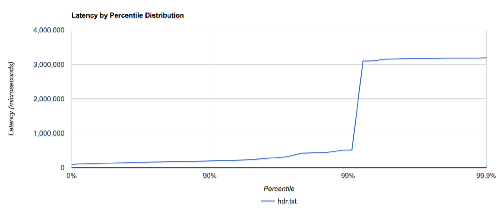
Y Axis

Recall that the samples were scaled to microseconds so you should label the Y Axis as such (there’s a dropdown control on the page to specify the units). The value for the Y axis is the value from the Value column in the histogram data file.

X Axis

The X Axis is the percentile for the test. The actual value used for the X is the 1/(1-Percentile) column which is a nice way of converting small differences in the increasing precision into something that can be plotted.

Conclusion

Read through the links above to Gil’s articles and videos, it’s great material. The key thing for me was to understand the form of the data being recorded. Hopefully you have a better understanding of it now as well.